Notes on Control Strategies for Stair-Climbing Exoskeletons

Stair-climbing exoskeletons are designed to provide assistive torque and stability for users with reduced lower-limb strength, mobility impairments, or balance limitations, and are widely applied in elderly care, disability support, rehabilitation, and load-bearing tasks. By delivering targeted knee or hip assistance during critical phases of stair ascent, they help reduce joint load, enhance safety, and promote greater functional independence. Clinical studies have further demonstrated their potential to restore gait function, strengthen lower-limb musculature, and improve neuromotor coordination [1][2][3]. However, achieving stable and efficient assistance remains challenging due to complex human–robot interaction: the coupled dynamics depend heavily on user-specific factors such as body mass, muscle strength, neuromotor condition, gait patterns, and soft-tissue deformation, all of which introduce significant variability and uncertainty. As a result, stair-climbing exoskeletons must rely on dedicated and adaptive control strategies to ensure safe, timely, and user-specific assistance.

Traditional control methods such as PD/PID controllers are simple and robust, and have been widely used in commercial and industrial exoskeletons. Nonetheless, they are insufficient for addressing complex HRI challenges. The high interaction stiffness often causes discomfort or results in the user being “dragged” by the robot, and the controller is unable to adapt to variations in user mass or voluntary effort [4].

A computed torque control (CTC) approach has been employed in [5,6] to improve trajectory tracking performance in exoskeletons. Compared with PD/PID control, CTC compensates for the nonlinear robot dynamics and enables smoother and more responsive tracking. However, its performance strongly depends on accurate dynamic modeling. In practice, human–robot coupling, soft tissue deformation, and individual variability make the dynamic terms,, anddifficult to model precisely. Furthermore, many studies rely on simplified or offline dynamic models, limiting real-time applicability.

Impedance/admittance control is widely adopted in rehabilitation robotics to ensure compliant and safe interaction. Most works, however, rely on fixed-gain impedance parameters, making it difficult to simultaneously achieve “sufficient assistance” and “adequate muscle activation.” Fixed parameters also fail to adapt to changes in patient state such as fatigue or voluntary engagement [7].

Feedback and feedforward control each have inherent limitations. Feedback control reacts only after errors occur, leading to unavoidable delay, whereas feedforward control reduces such delay but requires accurate modeling. Since exoskeleton dynamics are uncertain and user-dependent, relying solely on either feedback or feedforward control is insufficient for high-performance rehabilitation [8].

Sliding-mode control offers robustness against uncertainties such as friction and modeling errors , but it requires careful gain tuning, may suffer from chattering, and is not ideal for slow human joint motion. Its ability to compensate for highly nonlinear human–robot interaction remains limited [9].

A common limitation across existing approaches is the lack of an integrated and holistic control framework. Many studies focus on kinematic gait reproduction while ignoring dynamic safety; others emphasize dynamic control but adopt overly simplified gait generation without biological plausibility. Fixed-gain impedance control cannot provide individualized assistance, and learning-based controllers are often detached from model-based dynamics, limiting interpretability and safety. Additionally, many works rely on simplified or offline dynamics—such as Lagrangian formulations—which are computationally expensive for high-DOF systems and cannot support real-time control (500–1000 Hz). Model-based approaches typically focus on trajectory tracking but do not adapt to patient state or learn unmodeled dynamics such as friction or soft tissue effects [10][11].

In recent years, learning-based methods (e.g., neural networks and data-driven dynamic modeling) have been introduced to compensate for uncertainties that traditional models cannot capture. These methods can identify unmodeled nonlinear dynamics—such as soft tissue deformation, friction, human–robot coupling variability, and inter-subject differences—directly from interaction data. For example, Yang et al. [12] incorporated neural networks to estimate residual dynamics that are difficult to model explicitly, enabling improved tracking across gait cycles and maintaining stability under time-varying disturbances. Such learning modules enhance adaptability to uncertainty and individual differences, enabling more natural and personalized assistance.

Therefore, integrating biologically plausible gait generation, real-time dynamic compensation using the Newton–Euler algorithm, and AI/learning-based residual modeling for adaptive human–robot interaction represents a promising research direction. This integrated framework can address key challenges in rehabilitation robotics, including natural gait reproduction, individualized assistance, and real-time, safe, and adaptive control.

Proposed Control Strategy

The proposed control strategy adopts a hierarchical outer–inner loop architecture to generate safe and adaptive assistance during stair climbing. A gait/trajectory generator first produces desired joint profiles based on kinematic modeling. The outer loop regulates task-level behavior through an impedance controller, shaping the interaction dynamics between the user and the exoskeleton and producing a task-consistent desired torque. In parallel, the inner loop ensures joint-level stability and precise tracking by combining model-based feedforward dynamics—computed via the Newton–Euler algorithm—with feedback terms such as PID or sliding-mode control. To address modeling errors, user-specific variability, and unmodeled dynamics, an AI-based residual compensation module estimates and counteracts the remaining disturbances in real time. The resulting torques from impedance, model-based feedforward, and AI residual compensation are integrated and applied to the actuators, while inverse kinematics and sensing feedback update joint estimates for the next control cycle. This unified framework allows the controller to remain robust, adaptive, and compliant during human–robot interaction.

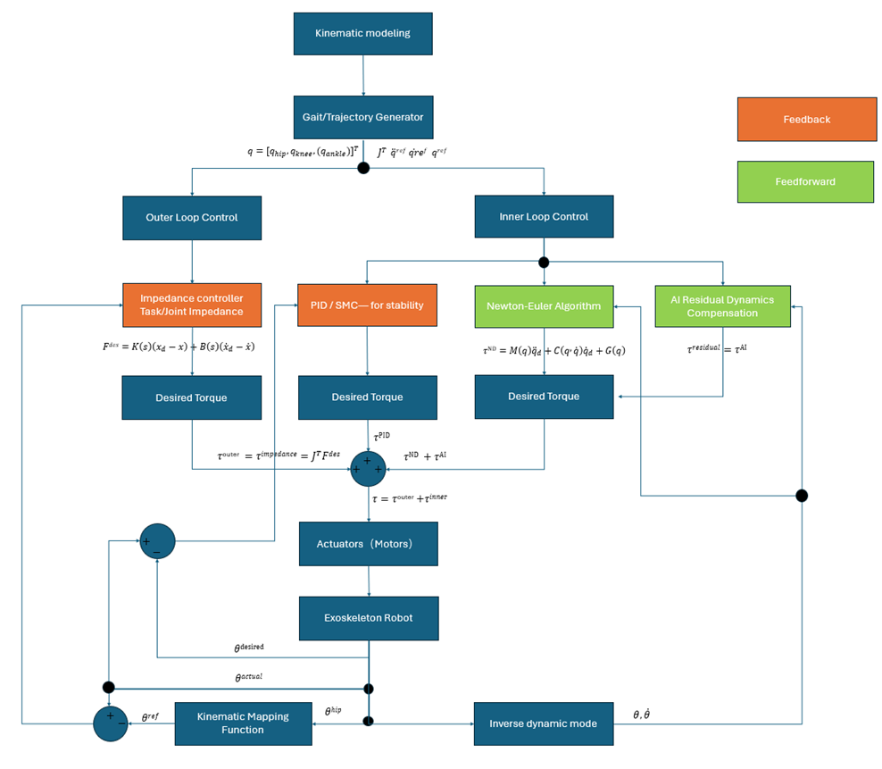
Fig1.Control diagram

Gait Generation based on Kinematic modeling

By using the exoskeleton’s own kinematic model, the robot can be made to “walk like a healthy person” even without a patient attached. This is achieved by inputting normative human gait data (e.g., joint angles or foot trajectories) and combining it with the robot’s kinematics (link lengths and joint DOFs) to generate a biologically plausible, robot-executable gait trajectory q_d (t)or x_"foot" (t).Such a trajectory can later be used as the patient’s target gait, an initial rehabilitation template, or a baseline for AI-based or adaptive control algorithms.

At first,we could Establish the kinematic model of both the robot and the human. A simplified lower-limb model with 2R or 3R joints (hip, knee, and optionally ankle) can be constructed. The joint variables are defined as：

q=[q_hip,q_knee,(q_ankle)]^T

and the geometric relationships are described using the link lengths l_"thigh" and l_"shank" . The foot-end position can then be expressed as

x_foot=f(q),y_foot=g(q)

Based on human thigh and shank lengths, an “equivalent human model” can be defined, or anthropometric measurements obtained experimentally (e.g., thigh and shank lengths) may be used directly. This step establishes the geometric basis required to compare and map human gait data to the robot.The subsequent modeling process can be carried out using the Denavit–Hartenberg (DH) convention.

Normal human gait trajectories can then be obtained by collecting experimental motion data, such as using motion-capture markers to record hip, knee, and ankle joint angles over time q_"human" (t), or by extracting the foot-end trajectory x_"foot,human" (t).

To save time, publicly available gait databases may also be used, where typical normative gait patterns can be imported and subsequently normalized. Many gait studies additionally provide averaged joint-angle curves derived from healthy populations. Regardless of the data source, these methods allow us to obtain a reference trajectory representing healthy human walking.

Although normal human walking exhibits variations in speed and step length, the gait cycle can be normalized to 0–100% to achieve temporal consistency. Each joint-angle or foot-end trajectory can then be smoothed and fitted using methods such as cubic splines, polynomial approximation, or CPG-based sinusoidal functions.This process yields a parameterized representation of the gait pattern:

In joint space:
q_human (s),s∈[0,1]" (gait phase)"

In task space (foot trajectory):
x_(foot,human) (s),y_(foot,human) (s)

The next step is to map the “human gait” onto the “robot gait,” typically through foot-trajectory imitation and inverse kinematics. When the robot’s structure is not identical to that of the human limb, it is common to use the human foot trajectory as the target:

x_(foot,d) (s),y_(foot,d) (s)

Inverse kinematics is then applied to the robot to compute the corresponding joint angles for each gait phase：

q_(robot,d) (s)=f_robot^(-1) (x_(foot,d) (s),y_(foot,d) (s))

n this way, the robot’s actual foot motion closely approximates that of a human. An advantage of this approach is that it does not require the robot’s joint angles to match the human joint angles exactly; instead, it only enforces similarity in the resulting foot motion, which is more biologically meaningful. This task-space formulation also makes it easier to incorporate variations such as obstacle avoidance or changes in step length.

Once the robot gait reference q_("robot" ,d) (t)is obtained, it can be used directly as a joint-space reference trajectory and tracked using PD/PID control, impedance control, or inverse dynamics control. For healthy subjects, this allows us to verify the robot’s ability to reproduce a normal gait pattern. For patients, the generated trajectory can serve as an ideal gait template for rehabilitation.
Alternatively, the same reference can be used in task-space control. By applying the Jacobian relationship x ̇=Jq ̇and the force mapping τ=J^T F, Jacobian-based or impedance-based controllers can be implemented to achieve compliant interaction between the foot and the ground.

Newton Euler method with spatial dynamics representation, which provides efficient calculation suited for a real-time control environment

To enable real-time online learning of the dynamic residual model, the computationally efficient Newton–Euler recursive algorithm can be adopted as the baseline dynamics for the learning module.

Since movements can vary rapidly during moving, real-time generation of inverse-dynamics torque is essential for achieving compliant interaction and precise assistance. This structure allows the exoskeleton to perform inverse dynamics computations at high control frequencies and supports online adaptive control. Given that the control loop typically operates at 500–1000 Hz, all dynamic computations must be completed within 1–2 ms. Only the efficiency of the Newton–Euler (NE) algorithm can support such real-time requirements as well as online learning modules such as disturbance learning and neural-network-based compensation.

It computes joint torques using force/torque balance through a forward recursion followed by a backward recursion: the forward iteration computes the angular velocity, angular acceleration, linear velocity, and linear acceleration (including gravity) of each link, while the backward iteration computes the inertial forces, inertial moments, and ultimately the torques required at each joint.

The key advantage of this method lies in its extremely high real-time performance, which is essential for inverse dynamics control where torque must be computed within 1–2 ms. In addition, the approach is highly modular and easily extensible; adding a new link does not require re-deriving the full dynamic model but only extending the recursive chain. From the robot’s kinematic model, the NE algorithm directly utilizes the homogeneous transformation matrices (typically obtained through DH parameters), the rotation matrices R_i^(i-1), the displacement vectors p_i^(i-1), the centers of mass r_(c_i ), the link inertia tensors I_i, and the joint type and joint axis direction z ̂.

Spatial dynamics representation refers to expressing rigid-body kinematics and dynamics using 6D spatial vectors that unify linear and angular quantities, enabling a compact and computationally efficient formulation of the Newton–Euler algorithm.

For a rigid link i, the spatial velocity is represented as a 6-D vector:
V_i=[█(ω_i@v_i )],

where ω_iand v_idenote the angular and linear velocities, respectively.
The forward recursion of the Newton–Euler algorithm in spatial form is:
V_i=X_i^(i-1) V_(i-1)+S_i q ̇_i,

where X_i^(i-1)is the spatial transformation matrix and
S_iis the joint motion subspace.

The spatial acceleration of link i is computed as:
A_i=X_i^(i-1) A_(i-1)+S_i q ̈_i+V_i×(S_i q ̇_i ),

where
V×(⋅)denotes the spatial cross-product operator for motion vectors.

The spatial force transmitted through link i is computed using:
F_i=I_i A_i+V_i ×^* (I_i V_i)+∑_(j∈"child" (i))▒X_j^(i*) F_j,

where:
I_iis the 6×6 spatial inertia matrix,
V×^* (⋅)is the spatial cross-product operator for forces,
X_j^(i*)is the dual transformation matrix from child link j to i.

The joint torque required at joint i is obtained by projecting the spatial force onto the joint motion subspace:
τ_i=S_i^T F_i.

This leads to the standard inverse-dynamics expression of a robot manipulator:
τ=M(q)q ̈+C(q,q ̇)q ̇+G(q),

where M(q)is the inertia matrix, C(q,q ̇)represents the Coriolis and centrifugal terms, G(q)is the gravity vector, and τdenotes the joint torques.

The other methods for deriving robot dynamics are the Lagrange–Euler method.The Lagrangian approach constructs the Lagrangian function from the system’s kinetic energy Tand potential energy V:
L=T-V

and applies the Lagrange equation:
d/dt(∂L/(∂q ̇_i ))-∂L/(∂q_i )=Q_i

Although this formulation is compact and physically interpretable—automatically generating desirable dynamic properties such as symmetry of M(q)and skew symmetry of M ̇-2C—it is most suitable for theoretical derivations or low-DOF systems (1–3 DOF), where the equations remain intuitive and manageable.For high-DOF systems, the Lagrangian method becomes computationally expensive, as each joint introduces multiple partial and time derivatives. The derivation is globally coupled, meaning that any parameter change requires re-deriving the entire system.

Most importantly, the Lagrangian method is not suitable for real-time inverse dynamics, as computing
τ_L (t)=M(q)q ̈_d+C(q,q ̇)q ̇_d+G(q)
within a high-frequency control loop is too time-consuming for practical use.

In this work, the controller must generate inverse-dynamics torques online, and must also compute dynamic residuals in real time:
τ_"res" =τ_"measured" -τ_ND (q,q ̇,q ̈ )

Since robots often possess multiple degrees of freedom and exhibit strong kinematic–dynamic coupling, with DOFs commonly exceeding 2–3, the Newton–Euler method offers clear advantages over the Lagrange formulation in terms of computational efficiency, modularity, suitability for high-DOF systems, and real-time inverse dynamics computation.

Dual-loop Control strategies

Based on the requirements of exoskeletons for compliant interaction, personalized assistance, and high-precision trajectory tracking, and assuming that the robot is able to measure EMG signals or plantar pressure, a dual-loop control strategy can be constructed by combining the biologically plausible gait reference generated from kinematics (Chapter 1) and the real-time inverse dynamics based on the Newton–Euler formulation (Chapter 2). The proposed structure consists of an outer-loop adaptive impedance controller and an inner-loop learning-enhanced tracking controller, enabling the system to automatically adjust assistance levels according to patient engagement while maintaining high tracking accuracy.

The outer loop employs EMG-/pressure-based adaptive impedance control, where the impedance parameters K,Band the reference trajectory q_d (t)are updated in real time according to the patient’s active participation level. This achieves individualized assistance modulation. The inner loop consists of Newton–Euler inverse dynamics combined with sliding-mode or AI-based compensation. The inverse dynamics term τ_NDprovides model-based feedforward torque, while sliding-mode or PID/SMC control baseline,then AI compensates for unmodeled dynamics and external disturbances（residual）, resulting in a high-bandwidth and robust control action. The combined control torque is given by
τ=〖τ_outer+τ_inner=τ〗impedance+τ_ND (q,q ̇,q ̈_d )+τ(PID/SMC)+τ_redidual

The reference gait is generated from human joint trajectories q_"human" (t)and foot-end trajectories x_"foot" (s),y_"foot" (s), which are normalized, fitted using splines, and parameterized to obtain
q_ref (s),s∈[0,1]

This reference is then mapped to the robot using inverse kinematics:
q_d (s)=f^(-1) (x_foot (s),y_foot (s))

A personalized gait adaptation can be incorporated by using surface EMG and plantar pressure (FSR/insole sensors) as inputs to characterize patient engagement:
"Engagement"(t)=ϕ("EMG"(t),"Pressure"(t))

Gait features such as step length, knee flexion, toe clearance, and gait cycle duration are adjusted accordingly, yielding the personalized trajectory
q_d (t)=q_ref (t)+Δq("Engagement"(t))

This allows the robot to reduce assistance when the patient is actively contributing, and increase stability and support when fatigue occurs.
For impedance control, the foot-end impedance model is
F=K(s)(x_d-x)+B(s)(x ̇_d-x ̇)

where K(s)is stiffness and B(s)is damping. The adaptive parameter update laws based on EMG and pressure are
K(s)=K_0+α_k (1-"Engagement"(t))
B(s)=B_0+α_b ("Pressure"(t))

High engagement reduces stiffness, while low stability or insufficient force increases damping, allowing the robot to enhance support. The outer loop therefore enables dynamic adjustment of gait and impedance characteristics according to people’s capability, realizing an Assist-as-Needed strategy.
In the inner loop, the Newton–Euler recursive algorithm computes the inverse dynamics:
τ_ND=M(q)q ̈_d+C(q,q ̇)q ̇_d+G(q)

PID and AI-based approaches are incorporated to further improve tracking performance.
For sliding-mode control (SMC), the tracking error is

e=q_d-q

and the sliding surface is
s=e ̇+λe

The SMC compensation torque is
τ_SMC=-K_s "sat"(s/ϕ)

If we use Iterative Learning Control (ILC) , which is suitable due to the periodic nature of gait, the update law is
τ_ILC^{((k+1))=τ_ILC}((k))+Le^((k)) (t)

allowing the controller to learn residual dynamics across repeated gait cycles.
Combining these components, the final control law becomes
τ_inner=τ_ND(q,q ̇,q ̈_d )+τ_(PID/SMC/ILC)+τ_residual

where τ_IDprovides dynamic compensation, τ_SMCensures stability and robustness, and τ_ILCimproves accuracy through cycle-to-cycle learning. The trajectory q_d (t)is supplied by the gait-generation module and the adaptive outer loop.

AI-Enhanced Dynamics and Adaptive Control

Building upon the kinematic modeling, dynamic modeling, and dual-loop control architecture established in previous Chapters, AI techniques can be employed to learn unmodeled dynamics, human–robot interaction behavior, and individual subject variability, thereby improving assistance accuracy, safety, and overall intelligence. Exoskeleton systems inherently involve complex nonlinearities (compliant contact, soft-tissue deformation, friction), inter-subject differences (leg length, muscle strength, pathology), environmental variability (different terrains and gait speeds), and human-interaction uncertainties (unknown patient force input, fatigue). As a result, conventional model-based control combined with fixed impedance cannot fully address these uncertainties. The primary role of AI is therefore to augment the dynamic model, capture patient-specific characteristics, and optimize control parameters.
During dynamic modeling, factors such as friction, cable-driven transmission (if present), soft-tissue compression, variations in fit and wearing tightness, and patient-generated forces were not explicitly modeled. AI can be used to learn these residual dynamics using NN, GP, ESN, RNN, or other learning models:
τ_real=τ_ND (q,q ̇,q ̈)+τ_residual (q,q ̇,q ̈)

where the AI model aims to learn
τ_residual

Typical approaches include neural networks (NN), Gaussian process regression (GP), and radial basis function networks (RBF-NN). GPU computing is beneficial for accelerating neural-network training or online updates, allowing residual learning to operate within high-frequency control loops.
Thus, an AI-based residual model is obtained:
τ_res (q,q ̇,q ̈)≈τ_real-τ_ND

The control torque becomes
τ_inner=τ_ND+τ_PID+τ_residual

where NE provides a reliable model-based baseline, AI learns unmodeled effects (friction, foot–ground interaction, patient-generated forces), and the inner-loop controller (SMC/ILC) maintains system stability. Importantly, the AI model does not directly control the system; it only compensates for model errors, while stability is ensured by the conventional controller.
In addition, AI can be applied to patient intent recognition and strength estimation (Estimator for Adaptive Control). In the outer-loop Assist-as-Needed control, we previously used:
Engagement(t)=ϕ(EMG,Pressure)

which represents an empirical mapping. AI enables a more accurate estimation: a neural network or GP model can map EMG signals into muscle activation estimates, interpret pressure distribution into gait-phase and stability indicators, and classify whether the patient is “active” or “passive.” The controller then adjusts impedance parameters (K/B), gait parameters (step length, toe-lift height), and assistance magnitude (torque scaling) accordingly.

AI can also be used for online tuning of controller parameters (Adaptive Gain Tuning). The parameters used in SMC, ILC, and impedance control—such as K_s,λ,K,B—can vary with patient state, gait phase, fatigue level, or contact condition. Manual tuning is difficult, slow, and inconsistent. AI can adjust these gains using reinforcement learning (online gain adaptation), meta-learning (cross-patient generalization), or supervised learning (mapping states to optimal gains). The control structure remains unchanged, but the parameters become intelligently adaptive.
Furthermore, AI can be used for gait deviation prediction (feedforward compensation). Although human gait is approximately periodic, patients may exhibit slow foot clearance, delayed knee flexion, or ankle hyperextension. AI can predict future tracking errors 100–200 ms ahead:

e ̂(t+Δt)=f_NN (q(t),q ̇(t),e(t))

A feedforward compensation term can then be applied:
τ_ff=K_ff e ̂(t+Δt)

which significantly improves tracking performance.

Conclusion

For lower-limb exoskeletons, we have developed a comprehensive control framework that integrates kinematics-based gait generation, real-time dynamic modeling, a dual-loop control structure, and AI-enhanced learning modules. The research contributions can be summarized as follows:

(1) Kinematics-based Gait Generation
By establishing kinematic models for both the human limb and the exoskeleton, normal human gait data are mapped to robot-executable trajectories. This enables the generation of biologically plausible reference gait patterns, providing a fundamental template mobility enhancement.

(2) Real-time Inverse Dynamics Based on the Newton–Euler Method
A comparison between the Lagrange–Euler formulation and the Newton–Euler recursive algorithm highlights the superior computational efficiency of the latter. Thus, Newton–Euler dynamics is adopted as the inverse-dynamics solver to achieve millisecond-level torque computation, supporting real-time control and online learning modules.

(3) A Systematic Dual-loop Control Framework (Outer Loop + Inner Loop)
A coordinated control structure is proposed: the outer loop performs adaptive impedance regulation based on EMG and plantar pressure to realize personalized assistance; the inner loop combines inverse-dynamics compensation with PID/SMC/ILC  to enhance tracking accuracy and system robustness.

(4) AI-Enhanced Control Modules
Learning-based components are incorporated, including:

• Residual dynamics learning to compensate for unmodeled effects such as friction, human–robot coupling, and inter-subject variability;
• Patient-intent estimation from EMG and pressure data, enabling refined impedance adaptation and gait modulation strategies;
• Learning-based gain tuning and gait deviation prediction, allowing the controller to adjust parameters online and anticipate future motion errors.

Reference

[1] X. Wang, R. Zhang, Y. Miao, M. An, S. Wang, and Y. Zhang, "$\rm PI^{{\text{2}}}$-Based Adaptive Impedance Control for Gait Adaption of Lower Limb Exoskeleton," IEEE/ASME Transactions on Mechatronics, pp. 1-11, 2024, doi: 10.1109/TMECH.2024.3370954.
[2] N. Aliman, R. Ramli, and S. Haris, "Design and development of lower limb exoskeletons," Robot. Auton. Syst., vol. 95, no. C, pp. 102–116, 2017, doi: 10.1016/j.robot.2017.05.013.
[3] Li, J. Xu, Z. Li, R. Song, and Y. Kang, “Dynamic Locomotion Synchronization and Fuzzy Control of a Lower Limb Exoskeleton With Body Weight Support for Active Following Human Operator,” IEEE Trans. Cybern., pp. 1–14, 2025.
[4] Munadi, M. S. Nasir, M. Ariyanto, N. Iskandar, and J. D. Setiawan, “Design and simulation of PID controller for lower limb exoskeleton robot,” AIP Conf. Proc., vol. 1983, 2018.
[5] T. Nef, M. Mihelj, and R. Riener, "ARMin: a robot for patient cooperative arm therapy," Medical & biological engineering & computing, vol. 45, n. 9, pp. 887-900 , 2007.
[6] K. Nagai, I. Nakanishi, H. Hanafusa, S. Kawamura, M. Makikawa, and N. Tejima, "Development of an 8 DOF robotic orthosis for assisting human upper limb motion," In Robotics and Automation,1998, Proceedings 1998 IEEE International Conference on, vol 4, IEEE, 1998, pp. 3486-3491.
[7] A. M. Abdullahi, A. Haruna, and R. Chaichaowarat, "Hybrid Adaptive Impedance and Admittance Control Based on the Sensorless Estimation of Interaction Joint Torque for Exoskeletons: A Case Study of an Upper Limb Rehabilitation Robot," Journal of Sensor and Actuator Networks,
[8] D. A. Bristow, M. Tharayil, and A. G. Alleyne, "A survey of iterative learning control," IEEE Control Systems Magazine, vol. 26, no. 3, pp. 96 114, 2006, doi: 10.1109/MCS.2006.1636313.
[9] R. Fellag, T. Benyahia, M. Drias, M. Guiatni and M. Hamerlain, "Sliding mode control of a 5 dofs upper limb exoskeleton robot," 2017 5th International Conference on Electrical Engineering - Boumerdes (ICEE-B), Boumerdes, Algeria, 2017, pp. 1-6, doi: 10.1109/ICEE-B.2017.8192098.
[10] A. Alsaied, J. Wang and K. Li, "Hybrid Impedance-Iterative Learning Control for Rehabilitation Lower Limb Exoskeleton Robot," 2025 8th International Conference on Intelligent Robotics and Control Engineering (IRCE), Kunming, China, 2025, pp. 64-68, doi: 10.1109/IRCE66030.2025.11203177.
[11]C. Xiao, Q. Chen, H. Shi and G. Gao, "Adaptive Repetitive Learning Control for Lower-Limb Rehabilitation Exoskeleton Robots," 2025 8th International Conference on Intelligent Robotics and Control Engineering (IRCE), Kunming, China, 2025, pp. 118-123, doi: 10.1109/IRCE66030.2025.11203121
[12] Y. Yang, D. Huang, and X. Dong, “Enhanced neural network control of lower limb rehabilitation exoskeleton by add-on repetitive learning,” Neurocomputing, vol. 323, pp. 256–264, Jan. 2019.